Sensor fusion is the merging of data from at least two sensors. In autonomous vehicles, perception refers to the processing and interpretation of sensor data to detect, identify, classify and track objects. Sensor fusion and perception enables an autonomous vehicle to develop a 3D model of the surrounding environment that feeds into the vehicle’s control unit.
While sensor fusion (fusion of data from different sensors) and perception (an online collection of information about the surrounding environment) is already in use in current ADAS and AD applications, the technology still has one major drawback: each detection is based on sub-optimal information (sensing data from the camera, radar, LiDAR, etc.), resulting in partial, or even contradictory information, which can lead the system to make a wrong decision.
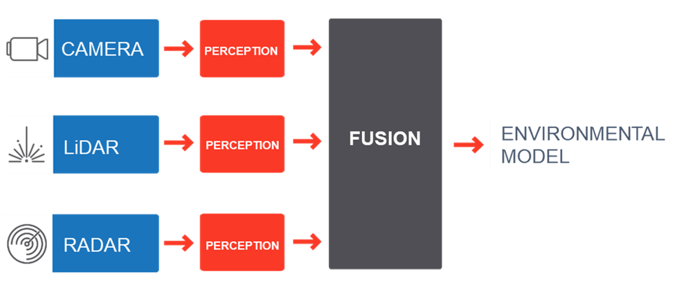
In a traditional object-level fusion approach, perception is done separately on each sensor (Figure 1). This is not optimal because when sensor data is not fused before the system makes a decision, it may need to do so based on contradicting inputs. For example, if an obstacle is detected by the camera but was not detected by the LiDAR or the radar, the system may hesitate as to whether the vehicle should stop.
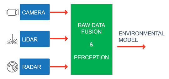
In a raw-data fusion approach, objects detected by the different sensors are first fused into a dense and precise 3D environmental RGBD model, then decisions are made based on a single model built from all the available information (Figure 2). Fusing raw data from multiple frames and multiple measurements of a single object improves the signal-to-noise ratio (SNR), enables the system to overcome single sensor faults and allows the use of lower-cost sensors. This solution provides better detections and less false alarms, especially for small obstacles and unclassified objects.
3D reconstruction generates a high-density 3D image of the vehicle’s surroundings from the camera, LiDAR points and/or radar measurements. By using the HD image from the vision sensor (camera), the algorithm divides the surroundings between static and dynamic objects. The LiDAR measurements on the static objects are accumulated over time, which allows the allocating of a larger portion of the distance measurements to moving targets. The acquired LiDAR measurements are further interpolated based on similarity cues from the HD image.
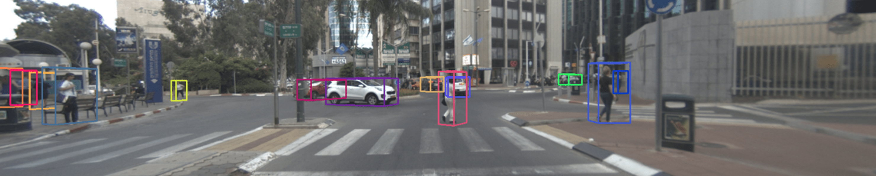
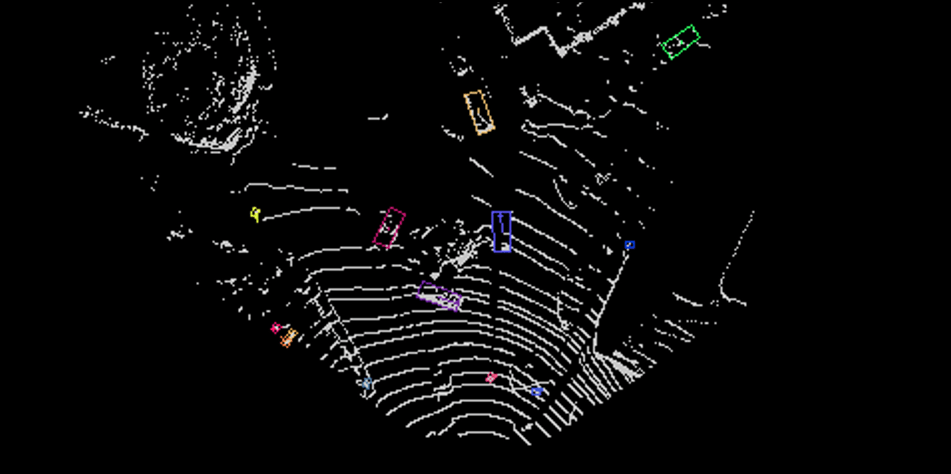
While LeddarVision’s raw data fusion uses low-level data to construct an accurate RGBD 3D point cloud, upsampling algorithms enable the software to increase the sensors’ effective resolution. This means that lower-cost sensors can be enhanced and provide a high-resolution understanding of the environment. The sample results of the 3D reconstruction algorithm for a camera and LiDAR are shown in Figure 3. The top picture represents the camera-only frame, the lower-left the original LiDAR point cloud and the lower-right the LeddarVision 3D reconstruction with upsampling.
For example, this method can be applied for low-density scanning LiDARs, as is demonstrated in Figure 3, thus enabling the use of a lower-cost scanning LiDAR, e.g., with 32 beams, instead of an expensive high-density 64-beam LiDAR, to achieve the required performance.
The RGBD model created through raw sensor fusion is sent to a state-of-the-art “RGBD object detection” module that detects 3D objects in a 4D domain. Meanwhile, the free space and road lanes are identified and accurately modeled in three dimensions, leading to an accurate geometric occupancy grid. This bird’s-eye-view grid of the world surrounding the AV is more accurate than using a camera-alone estimator. The RGBD model allows very accurate key-point matching in 3D space, thus enabling very accurate ego-motion estimation.

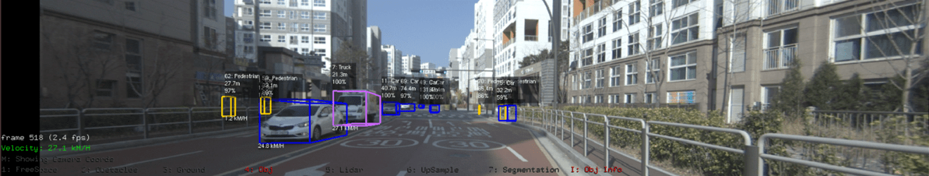
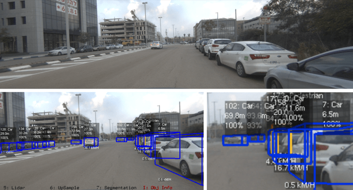
For safe driving, all objects on the road and in the vicinity must be detected, identified and tracked for proper path planning. An example is shown below. The system marks an object by placing a tight 3D bounding box around it, defining its position (x,y,z), dimensions (width, height, depth) and orientation (αx,αy,αz) with respect to the 3D scene and the car location. Furthermore, the bounding box is projected onto the image, and a 2D or 3D bounding box is marked on the image. Finally, the system classifies the object in one of the following categories: vehicle, pedestrian, cyclist or unknown. The “unknown” category is used to classify obstacles on the road that do not belong to any other category (e.g., a cat crossing the street, or a hole).
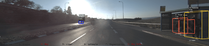
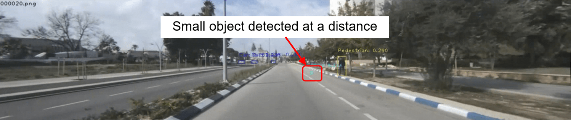
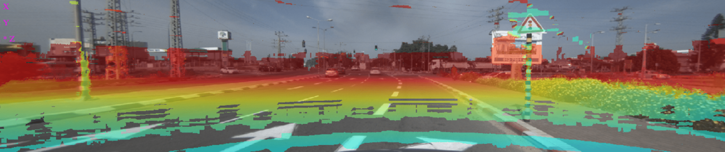
Raw data sensor fusion and 3D reconstruction provide more information that enables the detection algorithms to detect small objects farther than otherwise possible and smaller obstacles that would otherwise escape detection. It is this capability that provides the ability to safely drive faster and in more demanding conditions. LeddarVision’s novel RGBD-based detection utilizes the depth features of obstacles, allowing the recognition of never-before-seen obstacles. This technique helps bridge the gap between the outstanding performance of image-based deep-learning approaches for object detection and the geometry-based logic of an obstacle. The solution also reduces the number of false alarms, such as those that can occur due to discoloration on the road, reflections or LiDAR errors. The example in Figure 6 highlights the ability to detect such small obstacles even at large distances.
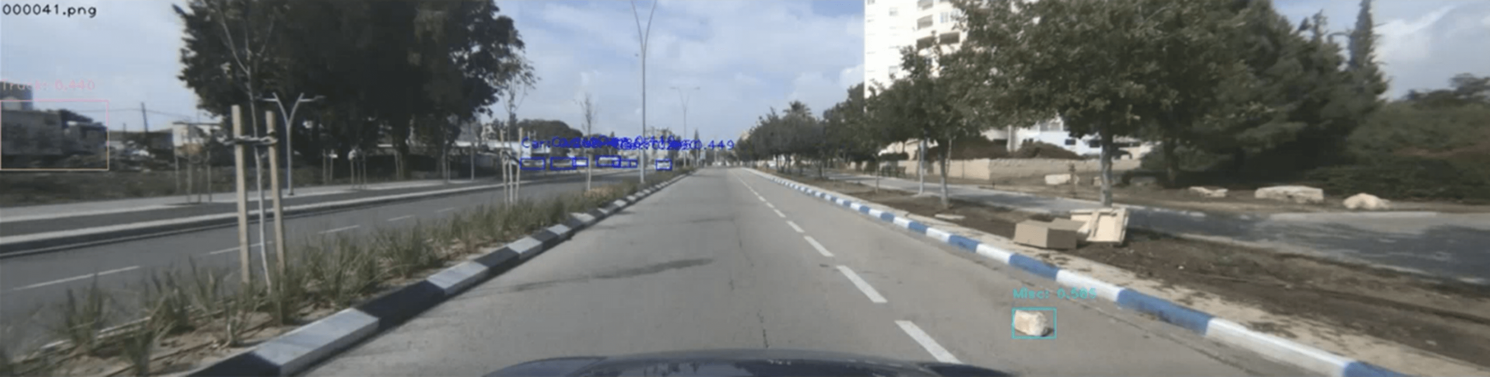
Figure 7 illustrates a small object on the road. Although it is still far away, the object is detected by the system, identified by a rectangle and classified as “unknown.” The obstacle is actually a rock on the road, as can be seen in Figure 8.
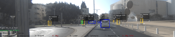
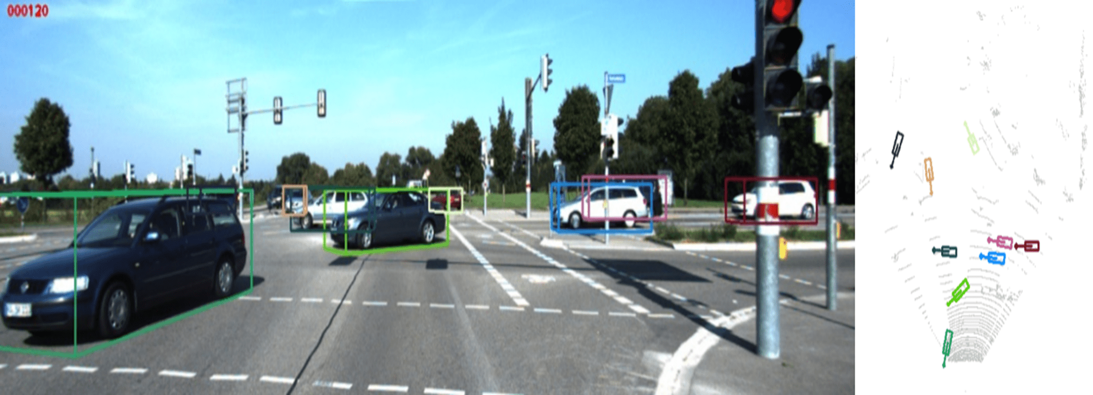
Once detected, each object must be assigned with velocity estimation. The algorithms track and follow each detected object’s motion path in 3D space by tracking the angular velocity through image frames and the radial velocity through depth-image frames. When Doppler radar data is available, this too is used. This allows the system to distinguish between dynamic and static objects. The method generates the 3D trajectory motion for dynamic objects, which will be used later for path planning and crash prevention. In the figure below, each 3D bounding box color represents a unique ID, and each vector in the bird’s-eye-view display represents the velocity of the object.
Advanced perception systems can also provide sophisticated algorithms for visual odometry self-localization, based on estimating the motion between every two consecutive frames of a camera image and LiDAR point cloud to create the motion vector and trajectory of the host car. This solution is based on LiDAR, camera, inertial measurement unit (IMU) and CAN-bus data, enabling operation in global navigation satellite system (GNSS) denied regions such as in a tunnel. If integrated with GNSS, the GNSS accuracy is then increased by an order of magnitude; for example, the module includes drift compensation based on GNSS readings and correction of GNSS reflections. Figure 10 shows an example of the ego-motion function (blue is ego-motion, pink is GNSS as ground truth).
The image was generated using only a single camera and a single LiDAR, with the vehicle driving approximately 500 meters.
Keypoints with a corresponding depth can be used for optimal ego-motion results, as shown in Figures 11 and 12. Keypoints are points in the frame that are static. In addition to their estimated depth, the ego-motion calculates the delta from the previous frame. The ones with the lowest estimated error are considered.


One of the significant outputs for ADAS and AD applications provided by a perception system such as LeddarVision is an accurate estimation of the free space available for the car to drive in, which is achieved by classifying each pixel in a “road / non-road” category. Proprietary algorithms take into account both HD-image and HD-depth map as created by the 3D-reconstruction block.
Free-space algorithm uses the front-view image to predict the per-pixel probability of a surface being drivable or not, using a deep convolutional neural network trained on extensive data collected over diverse and challenging scenarios. This prediction is projected onto a bird’s-eye-view perspective using LeddarVision’s non-linear bird’s-eye-view manifold estimation, which does not assume a single road plane. This leads to a more robust model of the road surface compared to a first-degree estimation of the road surface commonly used.

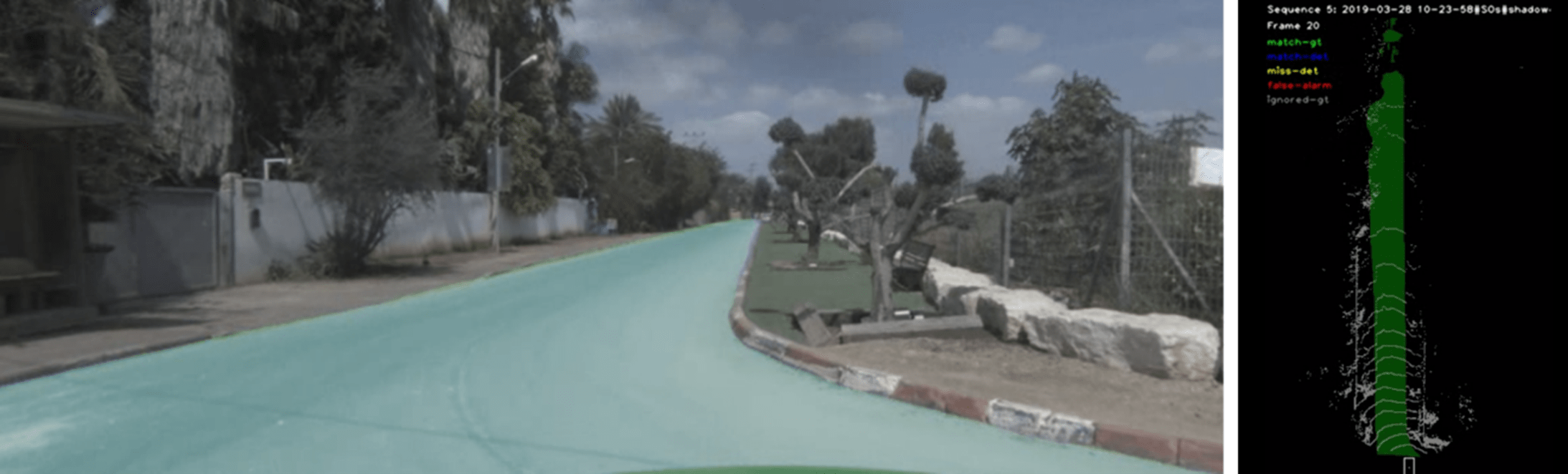
Advanced tracking algorithm utilizes temporal information to further improve detection results and to add a velocity vector to each object. This has a significant benefit in filtering out false alarms and improving all fields’ accuracy associated with an object’s detection, including velocity. As part of this process, each object is given an ID that can be tracked throughout a sequence which infuses measures of 2D detections with temporal measures, including ID switches, which are shown in Figures 15 and 16.
Free-space algorithm uses the front-view image to predict the per-pixel probability of a surface being drivable or not, using a deep convolutional neural network trained on extensive data collected over diverse and challenging scenarios. This prediction is projected onto a bird’s-eye-view perspective using LeddarVision’s non-linear bird’s-eye-view manifold estimation, which does not assume a single road plane. This leads to a more robust model of the road surface compared to a first-degree estimation of the road surface commonly used.
LeddarVision perception system can identify lane lines and divide the road into lanes, which is achieved through a mix of image processing algorithms to detect markers and supervised deep neural networks (DNN) to identify and classify the markers. The algorithm then generates a segmentation of lanes and lane borders, as shown in Figure 17. This feature is currently under development.
Once the surrounding lane markers are identified, the perception system analyzes and returns important information per lane marker, such as its type (dashed or solid), single or double and its color (white or yellow). Additionally, each lane is modeled using a polynomial fit with this model. Information on each lane’s width, known length and center is provided. Figures 18 and 19 show examples of this method.
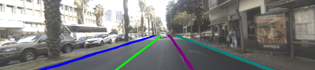
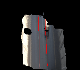 Figure 18. Bird’s-eye-view projection with a polynomial fit of the driving lane
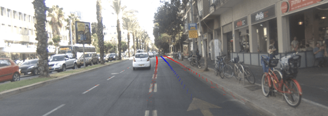 Figure 19. Driving lane and its middle visualization
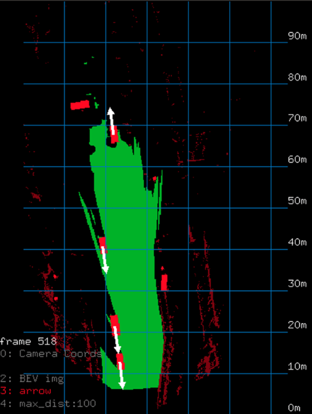
Occupancy grid is a bird’s-eye view of the vehicle’s surroundings, including the free space location and all surrounding objects, which enables path planning.
According to Wikipedia, “The basic idea of the occupancy grid is to represent a map of the environment as an evenly spaced field of binary random variables, each representing the presence of an obstacle at that location in the environment”.
Figure 20 below shows a typical example of an occupancy grid, where green areas represent free space, red areas represent objects and arrows represent velocity.
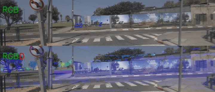
RGBD-based detection utilizes the scene’s image-based and depth-based features in parallel to accurately find all objects in the vehicle’s surroundings. This technique has several advantages:
The detector recognizes the following classes: vehicles (cars, trucks, buses, trains, etc.), and humans (a pedestrian, person sitting, cyclist, etc.).
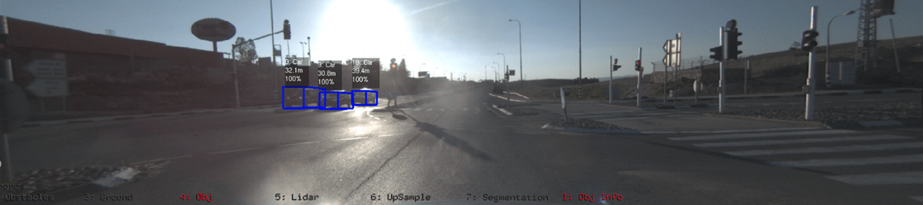
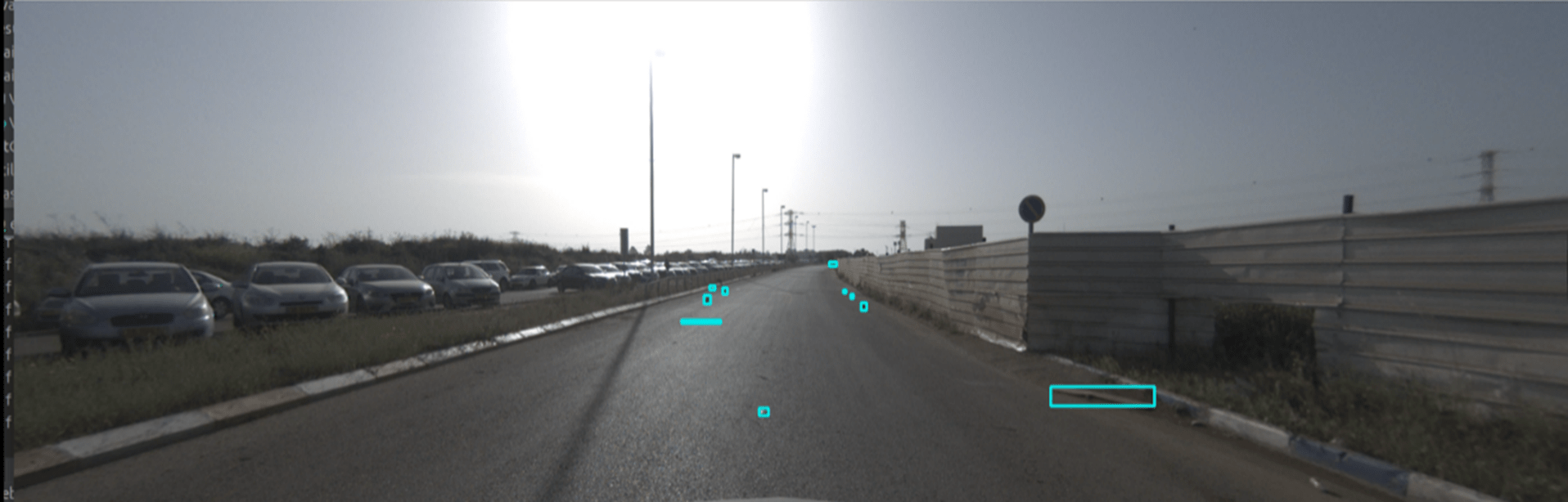
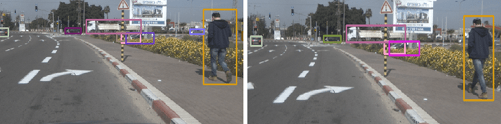
The following example compares camera-only detection working just on the RGB scheme and just on the camera, and fusion algorithms working on the RGBD. In the top picture, a poster installed on a fence features flat images of cars. Whereas the camera-only system detects cars on the poster (blue rectangles) that do not actually exist, the RGBD detection model can detect real cars that are located much farther away (top left in the bottom picture) and discriminate them from the 2D representations on the poster.
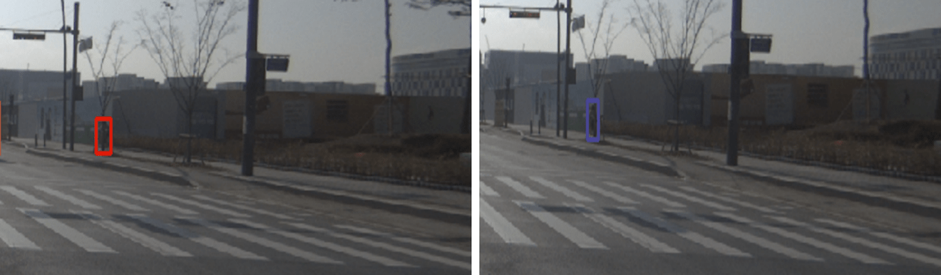
Another significant capability is that the system correctly detects partially occluded pedestrians, as illustrated on Figure 22, which demonstrates the system’s ability to perceive a pedestrian who is about to cross the road.
Each object detected by the perception system has a predicted position, size and orientation. The results of these predictions depend on the amount and accuracy of the LiDAR points returned from each object. LeddarVision perception system’s algorithm relies on a neural network’s accurate predictions. Also, a non-machine learning (ML) fallback option is used in cases of high uncertainty.
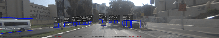
The following four figures show the advantage of detecting 3D objects assisted by the 3D reconstruction algorithm in low-visibility cases.